Intel® performance analyze tools

Intel VTune™ Amplifier XE Performance Profiler

The presentation can be downloaded here.

• provides information on code performance
• for users developing serial and multithreaded applications
• on Windows* and Linux* operating systems
• on Windows systems, the VTune Amplifier XE integrates into Microsoft Visual Studio* software and is also available as a standalone GUI client
• on Linux systems, VTune Amplifier XE works only as a standalone GUI client
• on both Windows and Linux systems, you can benefit from using the command-line interface for collecting data remotely or for performing regression testing

Use the VTune Amplifier XE to locate or determine the following:

• The most time-consuming (hot) functions in your application and/or on the whole system
• Sections of code that do not effectively utilize available processor time
• The best sections of code to optimize for sequential performance and for threaded performance
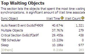
• Synchronization objects that affect the application performance
• Whether, where, and why your application spends time on input/output operations
• The performance impact of different synchronization methods, different numbers of threads, or different algorithms
• Thread activity and transitions
• Hardware-related bottlenecks in your code

Hotspot analysis

• Choose an analysis target.
• Choose the Hotspots analysis type.
• Run the Hotspots analysis to locate most time-consuming functions in an application.
• Analyze the function call flow and threads.
• Analyze the source code to locate the most time-critical code lines.
• Compare results before and after optimization

Рис. 2.1.

• Creating project If symbolic debug information is compiled into the executable it will help to find right lines of the code. But to analyze real application workflow it is recommended to compile with normal options
  

  
  Рис. 2.2.
• Choose the hotspots analysis type On the left pane of the Analysis Type window, locate the analysis tree and select Algorithm Analysis > Hotspots.
  

  
  Рис. 2.3.
• Analysis results
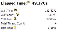
  • Note that CPU Time for the sample application is equal to 64.907 seconds. It is the sum of CPU time for all application threads. Total Thread Count is 3, so the sample application is multi-threaded.
    

    
    Рис. 2.4.
  • The Top Hotspots section provides data on the most time-consuming functions (hotspot functions) sorted by CPU time spent on their execution.
    

    
    Рис. 2.5.
• Call stackSelect the initialize_2D_buffer function in the grid and explore the data provided in the Call Stack pane on the right.
  

  
  Рис. 2.6.
• Analyzing the results
  • 

    
    
  • 

    
    
• Analyzing the results
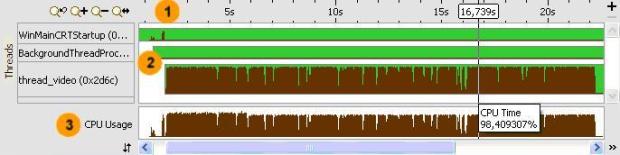
  1. Timeline area. When you hover over the graph element, the timeline tooltip displays the time passed since the application has been launched.
  2. Threads area that shows the distribution of CPU time utilization per thread. Hover over a bar to see the CPU time utilization in percent for this thread at each moment of time. Green zones show the time threads are active.
  3. CPU Usage area that shows the distribution of CPU time utilization for the whole application. Hover over a bar to see the application-level CPU time utilization in percent at each moment of time.
• Analyzing the code
  

  
  Рис. 2.7.
  • 1 –source code 2 –assembler
  • 3 –processor time,
  • 4 и 5 – useful markers and scroll controls to identify problem code
• Comparing the results
  • Specify the Hotspots analysis results you want to compare and click the Compare Results button
    

    
    Рис. 2.8.
  • 

    
    Рис. 2.9.
    • 1 – time difference
    • 2 – before the optimization (first version)
    • 3 – after the optimization
• Locks and waits analysis Other kind of analysis are provided in a similar way
  

  
  Рис. 2.10.
• Performing the analysis After the analysis you will be given an information according to the analysis type choosen
  

  
  Рис. 2.11.
  

  
  Рис. 2.12.
• Analyzing the results
  • Results are also could be viewed with the program call stack
  • 1 – corresponding object, 2 – processor usage,
  • 3 – wait cycles count
  

  
  Рис. 2.13.
• Analyze the code
  

  
  Рис. 2.14.
  • 1 – source code, 2 – processor usage,
  • 3 – wait loop count,
  • 4 - navigation
• Comparing the results
  

  
  Рис. 2.15.
  1. wit loop difference,
  2. wait loop count before,
  3. wait loop count after the optimizations,
  4. loop count difference,
  5. loop count
  6. loop count

Useful events

• CPU_CLK_UNHALTED.CORE – processor clock ticks
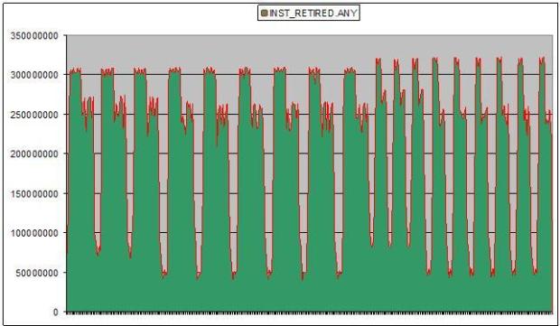
• INST_RETIRED.ANY – number of instructions been executed
• BUS_TRANS_ANY.ALL_AGENTS – bus transaction count
• L2_LINES_IN.SELF.DEMAND –L2 cache misses.
• BR_INST_RETIRED.MISPRED – mispredicted branch count

Рис. 2.16. Memory access time

Рис. 2.17. Memory access time

Рис. 2.18. Application performance analysis

Рис. 2.19. Application performance analysis

Useful compiler options

• /Od (-O0 for Linux) – no optimizations (used for debug).
• /O2 (-O2 for linux) – only default optimizations.
• /O3 (-O3 for linux) – some additional optimization set.
• /xO (-xO for Linux) – non-intel arhitecture optimizations.
• /Qipo (-ipo) - interprocedural optimizations.
• /Qparallel (-parallel) –autoparallelization.
• /Qopt-report (-opt-report)
• /Qopt-report-file
• /Qopt-report-phase
• /Qopt-report-help
• /Qopt-report-routine
• /Qvec-report [1/2/3]

Cluster tools

Рис. 2.20.

Intel Trace Collector & Analyzer

Cluster tools for enterprise applications with MPI.

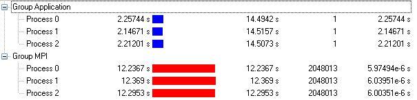
ITAC

Рис. 2.21.

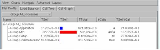
Similar analysis, but different application and different proposes

Рис. 2.22.

Рис. 2.23.

Рис. 2.24.

Рис. 2.25.

Рис. 2.26.