Элементы управления и динамика

Упражнения

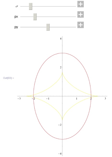
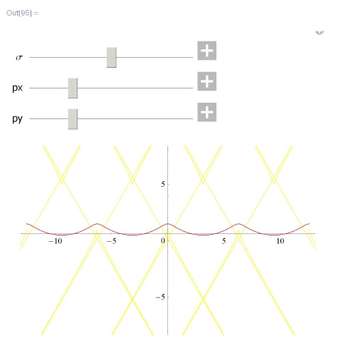
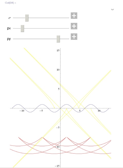
1. Для кривой визуализировать ее каустику (множество центров кривизны) и динамику волновых фронтов (эквидистант). Убедиться, что особенности волновых фронтов заметают каустику.

   >
   In[91]: =
          SetAttributes[wave, HoldFirst];
          wave [ {x_ [ t_, px_] , y_ [t_, py_]}, {px0_, pxmin_,  рхmах_},
                 {py0_, pymin_, pymax_}, {tmin_, tmax_}, {min_,  max_},
                  OptionsPattern[ParametricPlot]] : =
               DynamicModule q{?, s, v, a, n, q, k, caustic},
         Manipulate[
               ?[s_]:={x[s,px], y[s,py]};

   

   caustic[s_]:=? [s]+1/(k[s]) n[s];
                Show [ {
                   ParametricPlot[? [s], {s, tmin,  tmax}], 
                   ParametricPlot[caustic[s], {s, tmin, tmax},
                        Plotstyle -> Directive [Yellow] ] , 
                  ParametricPlot[? [s] +n[s] q,  {s, tmin, tznax} , 
                       Plotstyle -> OptionValue[PlotStyle]]
                } , PlotRange -> OptionValue[PlotRange], 
               AspectRatio -> OptionValue[AspectRatio] ] ,
            ] {{q, 0} , min, max} ,{{px, px0} , pxmin, pxmax} ,
            {{py, py0},  pymin, рутах} , Paneled -> False
         ]
      ]
   In[93]: =
            wave [{#2 Cos [#1] &[t, px] , #2 Sin[#2] &[t, py] } ,
                 {2, 1, 5}, {3, 1, 5}, {0, 2 ?}, {-1, 5},
                 {AspectRatio -> Automatic, PlotRange -> {{-3, 3}, {-4, 4}}, 
                      PlotStyle -> Directive[Red]} ]

   

   
   

   In[95]: = wave[{#l + #2 Cos [#2 + ?/2] &[t, px] ,
                       l + #2Sin[#l + ?/2] &[t, py]}, {0.5, 0, 2}, {0.5, 0, 2},
                    {-4 ? , 4 ? }, {-3 ?, З ? }, 
                    {AspectRatio -> Automatic,
                       PlotRange -> {{-4 ? , 4 ? } , {-8, 8}}} , 
                      PlotStyle -> Directive[Red] ]

   

   
   

   In[94]: = wave[{#l &[t, px] , Sin[#2] &[t, py] } , {2, 1, 5} , 
                   {3, 1, 5}, {-4 ?, 4 ? }, {-20, 20}, 
                   {AspectRatio -> Automatic,
                    PlotRange -> {{-4?,  4?} , {-15, 15}}} , 
                   PlotStyle -> Directive [Red] ]

   

   
   

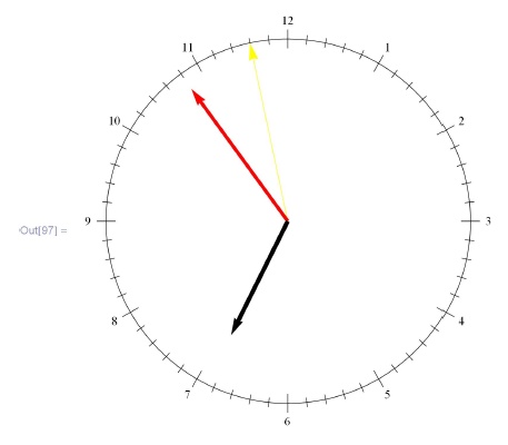
2. Смоделировать часы со стрелками.

   In[96]: = Dynamic[DateList [] , UpdateInterval -> 1]
   Out[96]= {2010, 2, 3, 18, 53, 57.5312500\}

   In[97]: =
      DynamicModule [ {?, ?, ?, ? = 0.05, ?1, ?} ,\\ Dynamic[ \\
       Graphics[
        {
          Circle[],
          Sequence @@ Table [if [Mod [i, 5] ==0, ?1 = ?,?1 = ?/2];
              ? = (2?)/(60) i; Line [{Cos [?] , Sin[?]}# & /@ {1 -?1, 1 + ?1}] ,
             {i, 0, 59}], 
          Sequence @@ Table [? =(2?)/4 - (2?)/(12)i ;
             Text[ToString[i] , (1 + 2?){Cos [?] , Sin [?]} ,
               Automatic], {i, 1, 12}],

   

   Arrow[{{0,0},{Cos[?], Sin[?]}}],

   

   Thickness[0.008],
             Arrow[{{0, 0}, (1-2?){Cos[?], Sin[?]}}],
             Black,
             ?=
               2?/4-
                  2?(1)/(12) - (Mod[DateList[] [[4]] , 12] + DateList [] [[5]] / 60) ;
               Thickness[0.01] ,
               Arrow[{{0, 0}, (1-6?) {Cos[?], Sin[?]}}]
           }
           PlotRange -> {{-1.2,  1.2}, {-1.2, 1.2}}, 
          AspectRatio -> Automatic] ,
        Update Interval -> 1
     ]
   ]

   Часы, смоделированные таким образом, на компьютере идут: